Пользовательского поиска

Графики индекса SP500, совокупной прибыли по отношению к денежной массе

SP E 1870

SP E 1930

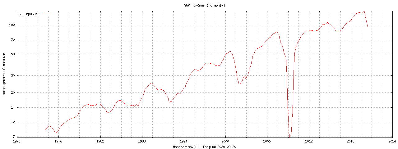
SP E 1974

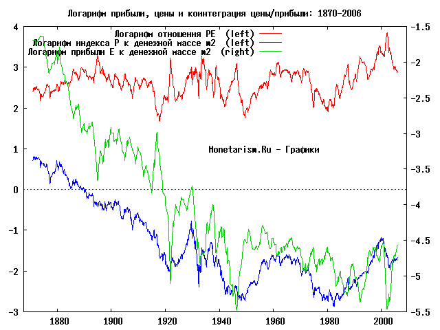
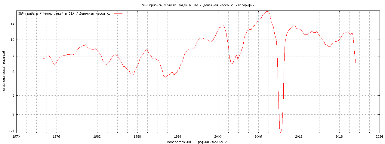
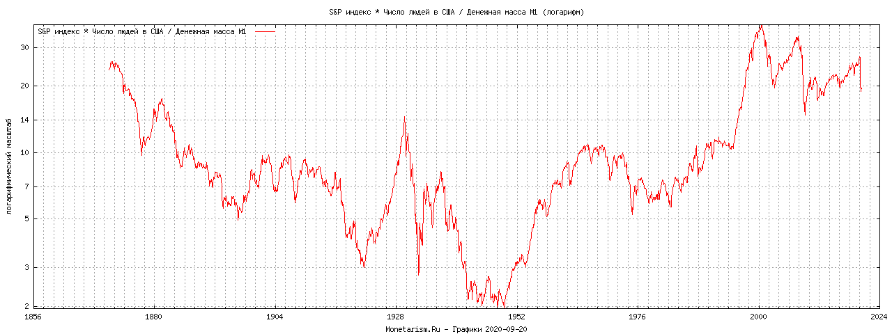
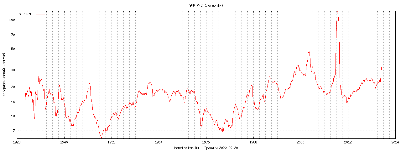
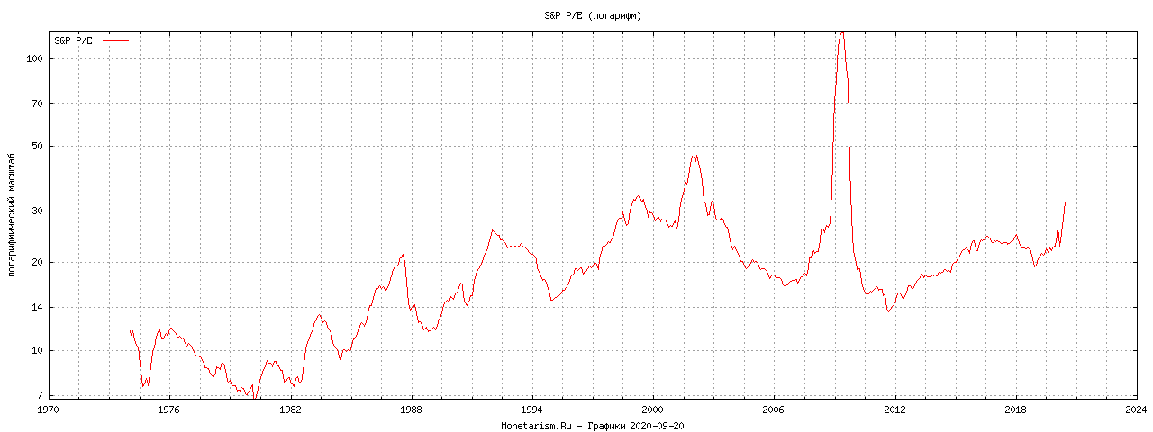
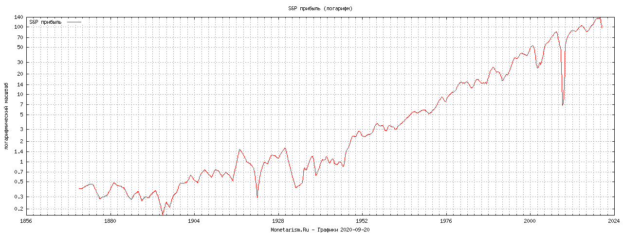
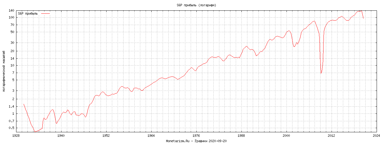
Графики отношения логарифма цены индекса и совокупной прибыли индекса с 1870 до 2006 года с учетом денежной массы М2 для американского рынка ценных бумаг (S&P 500)

Месячные данные. Обновление раз в год.

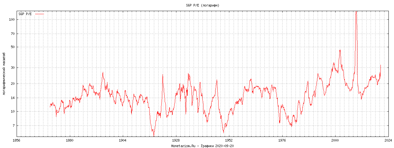
Коинтеграция коэффициента P/E

Step 3: cointegrating regression

Cointegrating regression - 
OLS estimates using the 1620 observations 1871:01-2005:12
Dependent variable: l_P_m2

      VARIABLE       COEFFICIENT        STDERROR      T STAT   P-VALUE

       const            2,36418          0,0351011    67,353  < 0,00001 ***
      l_E_m2            0,931760         0,00852611  109,283  < 0,00001 ***

  Unadjusted R-squared = 0,880685
  Adjusted R-squared = 0,880612
  Durbin-Watson statistic = 0,0171285
  First-order autocorrelation coeff. = 0,991544

Step 4: Dickey-Fuller test on residuals

Augmented Dickey-Fuller tests, order 12, for uhat
sample size 1607
unit-root null hypothesis: a = 1

   test without constant 
   estimated value of (a - 1): -0,0121636
   test statistic: t = -3,81563
   asymptotic p-value 0,002093

P-values based on MacKinnon (JAE, 1996)

There is evidence for a cointegrating relationship if:
(a) The unit-root hypothesis is not rejected for the individual variables.
(b) The unit-root hypothesis is rejected for the residuals (uhat) from the 
    cointegrating regression.

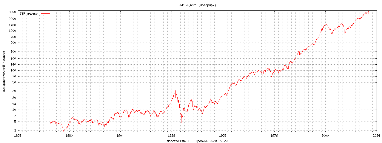
S&P chart SP 1870

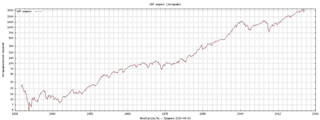
S&P chart SP 1930

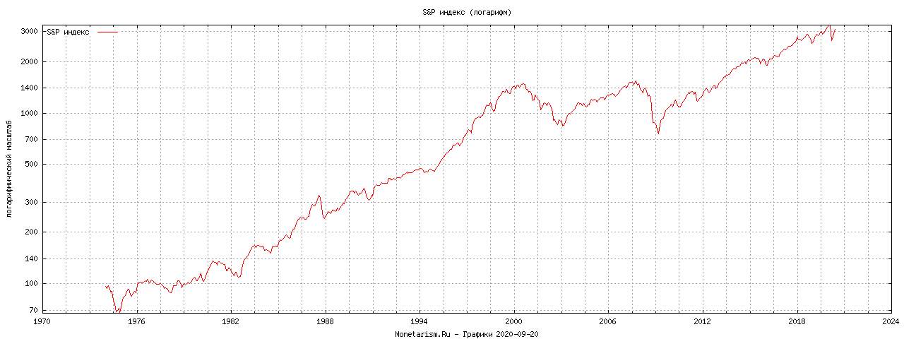
S&P chart SP 1974

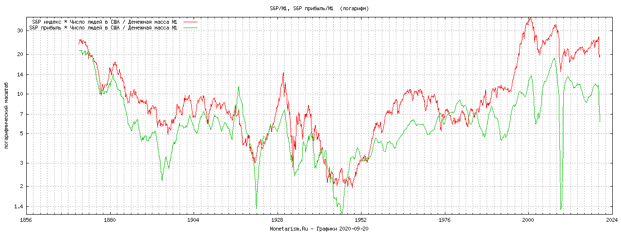
S&P*nPeople/M1 chart SP 1870

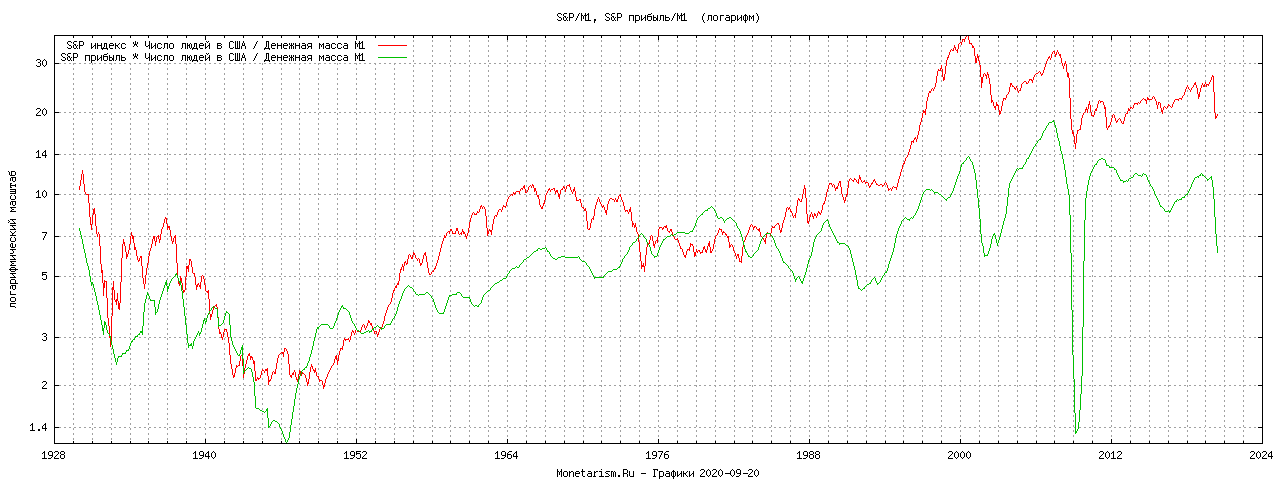
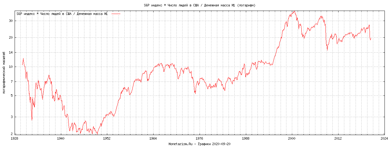
S&P*nPeople/M1 chart SP 1930

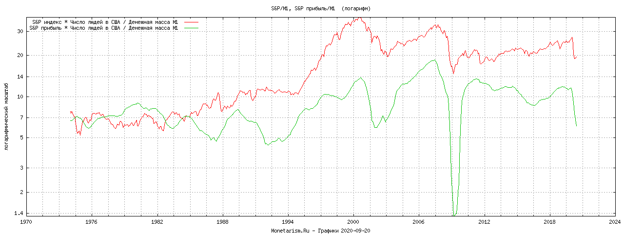
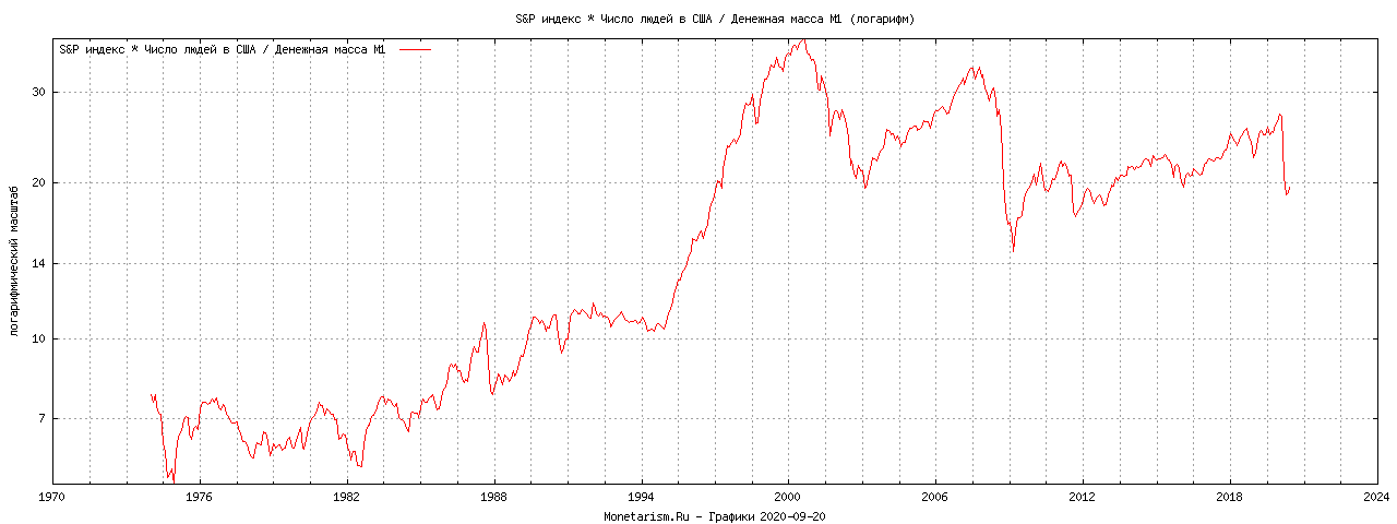
S&P*nPeople/M1 chart SP 1974

S&P P/E 1870

S&P P/E 1930

S&P P/E 1974

S&P Earnings 1870

S&P Earnings 1930

S&P Earnings 1974

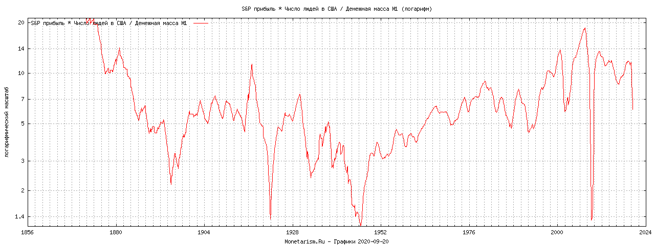
S&P Earnings*nPeople/M1 1870

S&P Earnings*nPeople/M1 1930

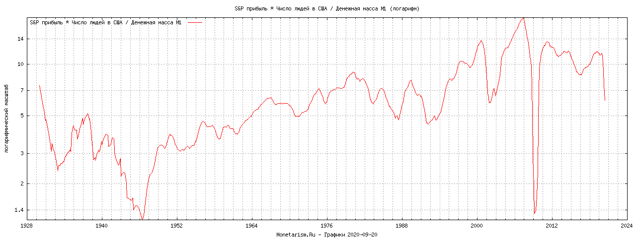
S&P Earnings*nPeople/M1 1974